The Impact of Actuarial Products on Retirement Outcomes

Introduction

Actuarial products exist to deal with the probabilities of unknown lifespans. These products are a form of risk pooling: The “winners” collect from the pool which only works if there are corresponding “losers” who pay for it. In reality, the pool consists of separate policyholders of the insurance company, but another way of looking at it is as a pool of one’s own different lifespan probabilities. All of the versions of “you” that pay the full amount of life insurance premiums and live a long life pay for the versions of “you” that meet an early death and collect the benefit. It works similarly for life income annuities where the “you” that dies shortly after purchasing the annuity funds the “you” collecting payments well past life expectancy. This is the point of view adopted in this article for exploring the effects of actuarial products on retirement outcomes.

Life insurance allows wealth to be transferred from outcomes with long lifespans to outcomes with short lifespans. Conversely, life income annuities allow wealth to be transferred from outcomes with short lifespans to outcomes with long lifespans. The ideal is to use these products to reduce the variability of outcomes due to the probabilities of different lifespans.

Methodology

The case study in this article is roughly based on the case study presented by Wade Pfau in his book Safety-First Retirement Planning: An Integrated Approach for a Worry-Free Retirement in the chapter on Life Insurance. That case study was mostly about using actuarial products to improve outcomes by mitigating risks when combined with an investment portfolio. This article is focused on looking at the impact of the actuarial products themselves. To this end, many aspects of the case study are simplified or eliminated.

The main simplification is that risk-free bonds yielding 3% interest per year are the only investment options available to all investors, including the insurance company. This removes the variability of market returns so that mortality is the only variable.

Another simplification is the use of a Roth account for retirement savings. According to Vanguard’s How America Saves 2025 , 86% of plans at Vanguard offered a Roth option in 2024, rising to 95% for larger plans. This makes it easier to account for everything on an after-tax basis.

Inflation is set at a constant 2% per year. Any taxes are paid at a 25% tax rate.

The mortality projections were obtained from the Alternative II (Best estimate) Cohort Life Tables of the Social Security 2025 Trustees Report . The 1985 cohort was used for both male and female since this would make them age 40 in 2025. The data from these tables are used for pricing both life insurance and life income annuities. All insurance products are fairly priced, meaning that all premiums paid and their earnings will be paid out in full based on the mortality probabilities.

Starting at retirement, accounts are spent down at a fixed amount adjusted annually for inflation that will lead to account depletion at age 110.

Also borrowed from Wade Pfau’s case study is the use of Lifetime Discounted Spending Power as a way to measure alternatives. The sum of all spending discounted back to the beginning of the case study using the 3% risk-free rate of return gives the Spending Power Present Value. “Spending” includes scheduled spending from accounts and annuity payments. Any account balances or death benefit received at joint longevity is considered “spent” at the death of the last spouse. Paying taxes and premiums is not considered “spending.”

Base Case

The Base Case starts with Mike and Fran, a 40-year-old male and female couple planning for retirement at age 65. Mike works for an income and Fran does not. This arrangement was chosen because life insurance is more expensive for males and life income annuities have a higher payout for males, but the roles could just as easily be reversed.

Mike currently has $45,000 in a Roth account. He will contribute $17,625 per year to the Roth account from ages 40-49, with the amount increasing by inflation each year. From ages 50-64, he will contribute $23,250 per year to the Roth account, also with the amount increasing by inflation each year from age 40 ($28,342 at age 50).

Figure 1 - Base Case, No Life Insurance (Full Size)

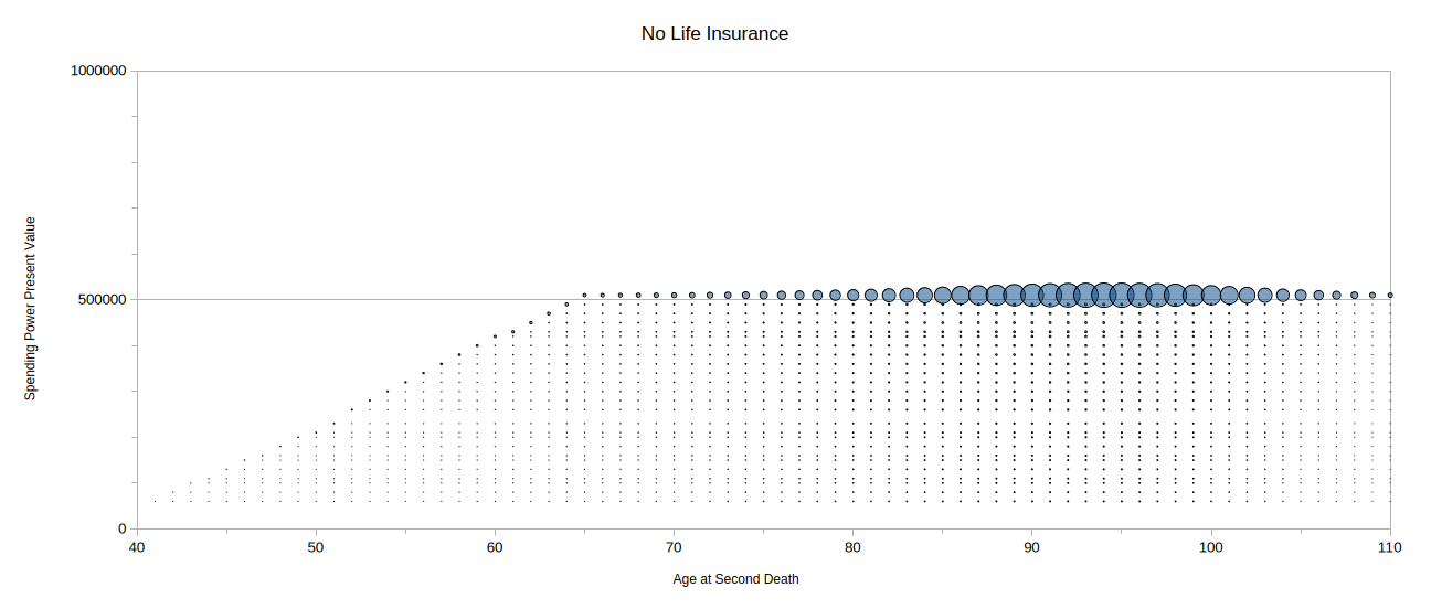
Figure 1 shows a bubble chart presenting the results of the Base Case. The x-axis of the graph is the age when the second spouse dies (joint longevity). The y-axis of the graph is the spending power present value discounted back to age 40, rounded to the nearest $10,000 so that close results can be combined. The bubbles represent the combined probability of getting a particular result. Interpreting the results, it is evident that the longer Mike remains alive (at least until retirement), the better the outcome. All of the small dots that look like rain falling from the big dots represent outcomes where Mike dies before reaching retirement, leaving Fran a widow with varying retirement prospects. The results of the Base Case show the worst-case extent of undesirable variability.

Proposal 1 - Term Life Insurance

This proposal starts with the Base Case described above but adds a 25-year level term life insurance policy for Mike from ages 40-64 with a face value of $500,000. Everything remains the same except Mike pays a fixed life insurance premium each year of $2,133, with the contribution to the Roth account reduced by the same amount.

Life insurance death benefits are tax-free when received. However, it is assumed that any death benefits will be put into a taxable account upon receipt. This creates a tax drag going forward of annually taxable interest.

Figure 2 - Proposal 1, Term Life Insurance (Full Size)

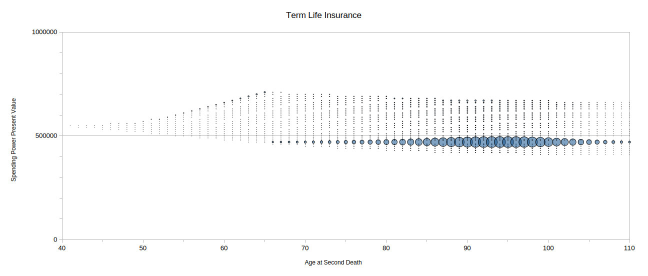
Figure 2 shows a bubble chart with the results. The straight row of larger circles in retirement are the outcomes where Mike lives until retirement. All of the other dots represent outcomes where Mike dies before reaching retirement and Fran receives a life insurance payout. The combination of an insurance payout and some amount of retirement savings always starts out higher than the full amount of retirement savings, but the tax drag of having the life insurance proceeds in a taxable account eventually pulls some of the widow’s results below the “default” case of Mike living to retirement. The cost of the widow’s benefits are also evident in the reduced full retirement savings results compared to the Base Case. Overall, this is a marked improvement over the variability of the Base Case.

Proposal 2 - Whole Life Insurance

This proposal also starts with the Base Case but adds a whole life insurance policy for Mike with premiums paid from ages 40-64 and a face value of $500,000. The premium for the policy is a fixed $7,962 per year, with the contribution to the Roth account reduced by the same amount.

Figure 3 - Proposal 2, Whole Life Insurance (Full Size)

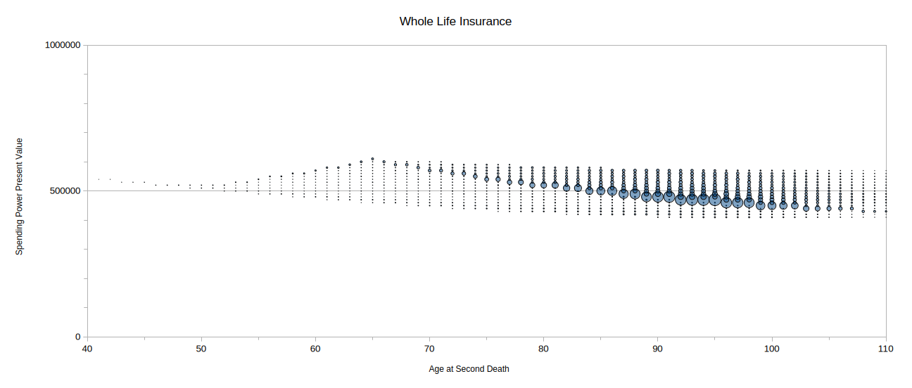
Figure 3 shows the results. The largest circle at each age represents the outcome of Mike being the last to die at that age. All of the rest of the bubbles are outcomes where Fran outlives Mike. The longer Mike lives, the less valuable the fixed life insurance payout becomes due to the time value of money.

The outcomes where Mike dies before retirement create the grid of small dots on the graph. The results of reaching retirement will full retirement savings and an intact insurance policy are overlaid on top of this grid in the shape of a declining triangle starting from the top bubble at age 65. The effect of ongoing life insurance is evident in this graph, with spending power starting relatively high for short lifespans and decreasing with increased longevity. For comparison, refer to the row of large bubbles in Figure 2 that starts off at a lower value but then stays flat to maximum longevity. Again, this is a large improvement over the variability of the Base Case.

Proposal 3 - Term Life Insurance & Joint Life Annuity

This proposal starts with Proposal 1 but adds the purchase of a life annuity at retirement. The life annuity will provide a starting after-tax annual payment of $26,350 with a 2% annual cost of living adjustment. If Mike is the sole survivor at age 65, he will purchase a single life annuity with a payout of 5.27% for $500,000 from the Roth account. If both spouses are alive at age 65, they will purchase a joint life annuity with a payout of 4.11% for $641,119 from the Roth account.

If only Fran survives to age 65, the situation is more complicated. She will purchase a nonqualified single life annuity with a payout of 4.78% for $603,595 from the taxable account funded by the proceeds of the life insurance death benefit. After applying an exclusion ratio of 65.315% and deducting taxes, this will provide the after-tax annual payment of $26,350. If the taxable account does not contain enough money to purchase the full nonqualified annuity, funds from the Roth account will be used to purchase a tax-exempt single life annuity to make up the shortfall in the after-tax annual payment.

Figure 4 - Proposal 3, Term Life Insurance, Joint Life Annuity (Full Size)

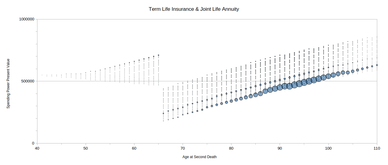
Figure 4 shows the results. The bottom row of large circles represents the outcomes where both spouses survive to retirement and a joint annuity is purchased. The slightly higher row of small circles represents the outcomes where Mike survives alone to retirement and purchases a single life annuity. The outcomes where Mike dies before retirement once again create the grid of small dots representing the varying amounts of retirement savings plus insurance proceeds that Fran brings into retirement as a widow. The effect of the annuities in retirement is shown by how the rows of outcomes slope upwards which indicates spending power starting lower at shorter lifespans and increasing with increased longevity.

Proposal 4 - Whole Life Insurance & Single Life Annuity

This proposal starts with Proposal 2 but adds the purchase of a single life annuity at retirement “covered” by the whole life insurance. The single life annuity will once again provide a starting after-tax annual payment of $26,350 with a 2% annual cost of living adjustment. If Mike survives to retirement, he will purchase a single life annuity with a payout of 5.27% for $500,000 from the Roth account. If Fran is the sole survivor at retirement, she will purchase a nonqualified single life annuity as described in Proposal 3.

If both spouses survive to retirement, this creates the possibility that Fran will need to purchase a replacement annuity in the event that Mike predeceases her. This process is no different for her than purchasing the annuity at retirement except the annual payment will have been adjusted over the years by the COLA.

Figure 5 - Proposal 4, Whole Life Insurance. Single Life Annuity (Full Size)

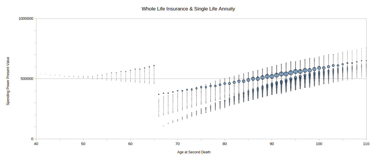
Figure 5 shows the results. The row of largest circles represents the outcomes where Mike is the last to survive. The declining time value of the whole life policy moderates the otherwise upward slope caused by the annuity. The bottom rows that look like ice cream cone scoops represent outcomes where both spouses survive to retirement but then Mike is the first to die. The higher up the “scoop” is on the ice cream cone, the longer Mike survived in retirement. The spending power drops at Mike’s death due to the need to purchase a replacement annuity. And finally, the usual grid of small dots represents the outcomes where Mike dies before retirement.

Proposal 5 - Whole Life Insurance & Joint Life Annuity

This proposal is identical to Proposal 3 with the exception of substituting a whole life insurance policy for the term life insurance policy. This is also identical to Proposal 4 with the exception of substituting a joint life annuity for the single life annuity when both spouses survive to retirement.

Figure 6 - Proposal 5, Whole Life Insurance. Joint Life Annuity (Full Size)

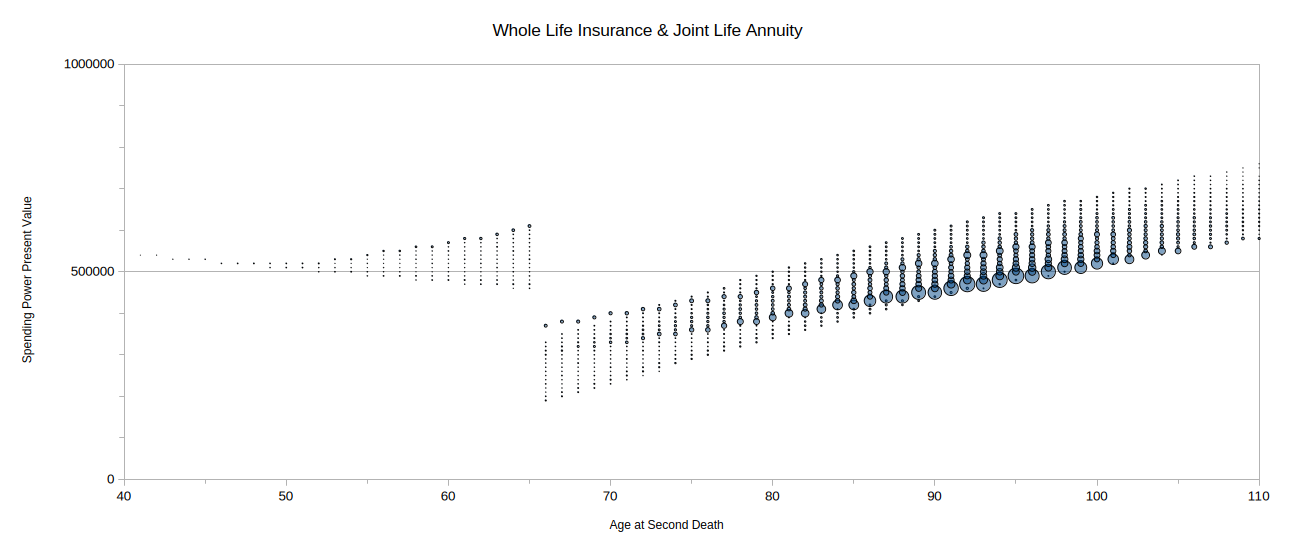
Figure 6 shows the results. The familiar grid of small dots is present, representing the outcomes where Mike dies before retirement and Fran buys a single life annuity. The bottom row of large circles represents the outcomes where both spouses survive to retirement, they purchase a joint life annuity, and Mike is the last to survive. The row somewhat above it of medium-sized circles represents the outcomes where Fran does not survive to retirement and Mike buys a single life annuity. The other circles larger than dots represent the outcomes that start as the “joint” outcome but Mike dies first and Fran collects the life insurance payout which she is then able to start investing and spending.

Analysis

While it is informative to see the distribution of probable outcomes due to the different combinations of life insurance and life annuities, it is also useful to compare the strategies to each other.

Figure 7 - Weighted Average Results (Full Size)

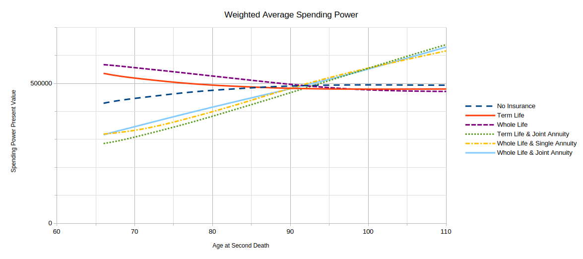
Figure 7 shows the weighted average of the outcomes at each joint longevity age for each strategy. Only the ages after retirement are shown. (It is important to note that the ages themselves do not have the same probabilities. The age with the highest combined probability is age 94 with a probability of about 5%. In contrast, age 79 and age 105 each have a combined probability of about 1%.) The graph shows that on average the whole life insurance options tend to outperform the term life insurance alternatives. The term life insurance options only outperform at well above average longevities, at least on the basis of the weighted average results. The standout performer is the combination of whole life insurance with a joint life annuity.

Figure 8 - Ideal Spending Profile (Full Size)

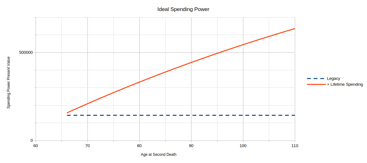
But what is the ideal result being sought for spending power with increasing joint longevity? Spending power is the sum of lifetime spending plus legacy. Presumably, the desired legacy is a level amount while the desired lifetime spending is smooth consumption with the total amount proportional to joint longevity. This means that ideally spending power should be equal to the desired legacy at minimum longevity and should be equal to the desired legacy plus the sum of the years of spending at maximum longevity. Figure 8 shows the ideal result of a level time value of legacy with smooth inflation-adjusted lifetime spending added on top. The graph illustrates the need for either a life annuity or an investment portfolio that grows faster than the time value of money or some combination of the two. A life annuity satisfies this need with guaranteed income.

Figure 9 - Worst-Case Results (Full Size)

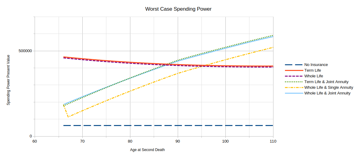
Looking at averages is only one part of the results. The variability of results is at least as important. Figure 9 shows the worst-case outcomes for each strategy. What is most evident from this graph is that the combination of a single life annuity with whole life insurance and the possibility of a separate survivor single life annuity creates significant downside risk. It is essentially making a wager that Mike will outlive Fran or at least have a very long lifespan. The insurance company takes on this risk with a joint life annuity, ensuring an average result.

Conclusion

The effects of actuarial products on retirement outcomes are not always obvious. It is too easy to focus on one aspect of a product that addresses a specific problem area. This article has taken a more comprehensive approach that leads to four findings:

First, it is important to consider the full array of possible outcomes. Some results may come as a surprise if not properly studied, especially the variability of outcomes.

Second, while not a novel idea, life insurance in pre-retirement is essential to ensure a successful retirement. The results of this case study show that both term life insurance and whole life insurance provide fairly similar consequences. This case study also shows that whole life insurance provides measurable upside at shorter longevities while only slightly underperforming at extended longevities.

Third, a life annuity is necessary to create the proper spending profile for retirement. While not considered in this case study, a market-based investment portfolio with a sufficiently high expected return can also serve this purpose but at the cost of introducing market risk. In contrast, a life annuity provides guaranteed income.

Finally, gambling on a single life annuity to address joint longevity introduces unnecessary variability in retirement outcomes. The needs of spending for joint longevity are best met with a joint life annuity.